
Virtual Towing Tank State-of-the-Art and Future Trends


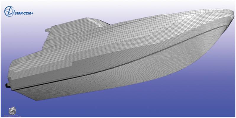 Fig. 5:Computational grid on the surface of a patrol boat.
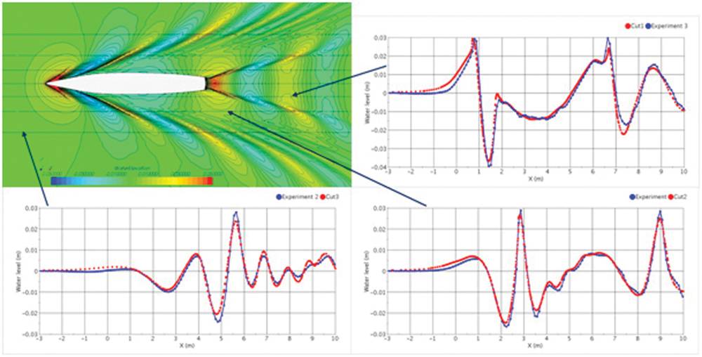
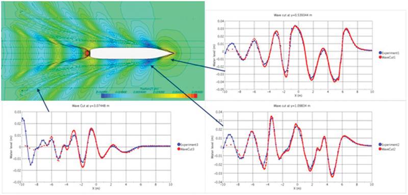 Fig. 1: Predicted wave pattern around KCS-hull at Froude-number 0.26 and comparison between predicted (red) and measured (blue) wave profiles along three longitudinal cuts.
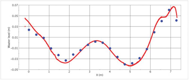 Fig. 2: Predicted profile of wetted hull surface for the KCS at Froude-number 0.26: simulation (red line) and experiment (blue dots).
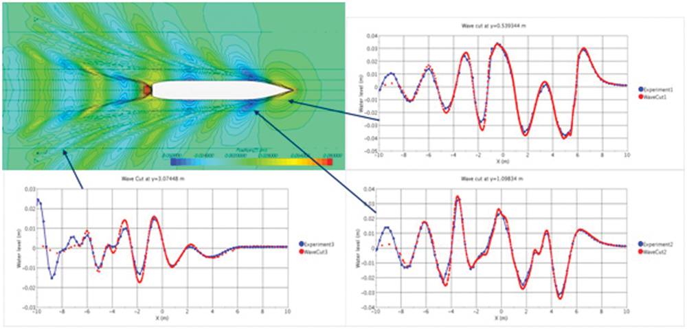
 Fig. 3: Predicted wave pattern around DTMB-hull at Froude-number 0.28 and comparison between predicted (red) and measured (blue) wave profiles along three longitudinal cuts.
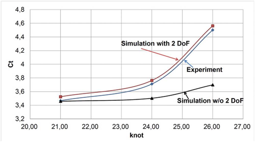
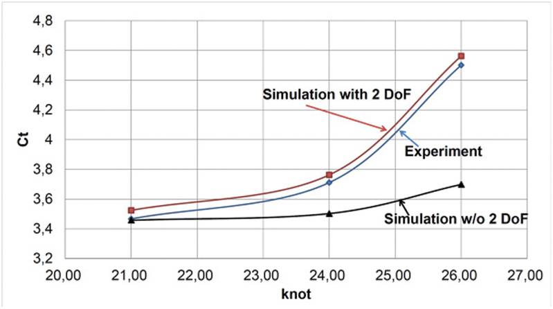 Fig. 4: Prediction of resistance of KCS-hull in fixed position and with free trim and sinkage, compared with experimental data for the free condition.


The use of computers to solve hydrodynamics problems in shipbuilding started in early days of scientific computing – as early as in aerodynamics and aerospace. Due to limited computing resources at that time, potential flow model was used in both aero- and hydrodynamics. However, while simulations based on Euler equations, Reynolds-averaged Navier-Stokes equations (RANSE) and most recently partially resolved Navier-Stokes equations (so-called “large-eddy” – LES – or “detached-eddy” – DES – simulations) have become established tools in aerodynamics, ship hydrodynamics is still predominantly simulated using methods based on potential flow. There are good reasons for this:
• The presence of free surface with its arbitrary deformation and breaking makes the simulation difficult and commercial software that can perform coupled simulation of flow and motion of floating bodies has only recently become available.
• The computational effort for simulations based on Navier-Stokes equations is several orders of magnitude larger than for methods based on potential theory.
Methods based on RANSE have been used in research institutions for marine applications for quite a while, but extensive use of such methods only recently become a commonplace. In addition to the need to account for flow features which potential flow model does not cover (turbulence, viscous effects, breaking waves etc.), the availability of inexpensive computer clusters and easy-to-use commercial software has greatly facilitated this trend. Also, new generations of engineers are being educated in computational fluid dynamics (CFD) and are thus eager to adopt these new simulation methods. Regular conferences and workshops dedicated to the use of CFD in marine engineering are also influencing this trend (e.g. NuTTS – Numerical Towing Tank Symposium, held every year and for the 15th time in 2012).
Although some people claim that simulations will replace experiments completely, we believe this will not happen any time soon. One reason is that CFD still uses models that need to be validated for each new application area (like turbulence and two-phase flow or phase change models). Also, some simulations – while in principle possible – would take too long to be performed with sufficient accuracy so experiments are the more efficient approach (like for maneuvering and sea-keeping problems). The combination of the two approaches is the best way towards optimum products: simulation can be used in early design stages and provides a wealth of information that helps understand the physics of the problem, while well-designed and instrumented experiments are needed to validate CFD tools.
However, there are many problems that can be solved today with CFD very efficiently with a satisfactory accuracy. Below are the elow results of several recent validation studies, before discussing industrial applications and future trends.
State-of-the-Art in Commercial CFD
All results presented here were obtained using new-generation software STAR-CCM+ from CD-adapco. It is based on finite-volume method and can use control volumes (CVs) of arbitrary polyhedral shape. This allows handling of complex geometries and changes in CV-topology since there are no limitations to the number of faces one CV can have. A range of turbulence models, an interface-capturing scheme for free surfaces, a cavitation model, moving and overlapping grids, sliding surfaces and a dynamic fluid-body interaction (DFBI) model are also available. Compressibility effects in both liquid and gas phase are accounted for. The software also contains a CAD-modeler and repair tools so that the body of flow domain can easily be obtained even if the ship is defined by the shell of hull surface. The computational grid defining CVs is created fully automatically and the user can prescribe the size of control volumes using line, surface and volume control parameters. The whole process from CAD to solution can easily be automated and saved in templates so that non-experts can perform parametric studies once the simulation is set up by a knowledgeable engineer. This also facilitates the use of optimization software (like FRIENDSHIP-Framework from Germanischer Lloyd) since it can automatically vary geometry and other parameters and perform CFD-simulations by executing templates with replaced geometry. More information about CFD that applies to most commercial software can be found in Ferziger and Peric (2003, 2008).
There are other software tools on the market that cover most of the above-named features to a varying level of detail and a new user is advised to check all options to find the best tool for particular purpose.
Validation of CFD for Marine Applications
The authors of this article were involved in several recent validation studies. Results from prediction of resistance, trim and sinkage of KCS-hull were presented at the Gothenburg-workshop in 2010 and will not be repeated in detail here (see Enger et al, 2010).We only note that the trend with varying Froude-number was well predicted for all three quantities, and that systematic grid refinement was used to demonstrate convergence towards a grid-independent solution. In particular, the resistance was predicted within 1% of the measured value on the finest grids (comprising around 3 million CVs) for all three hulls investigated at the workshop. Here only the results for wave profiles are given which were not presented at the workshop. Results from other contributors can be seen in Workshop Proceedings (Larson et al, 2010).
Figure 1 shows predicted wave pattern around KCS-hull (KRISO Container Ship) at Froude-number 0.26 (fixed position) and comparison between predicted and measured wave profiles along three longitudinal cuts. The simulation is performed in model scale with hull length of 7.2786 m, draft of 0.34177 m (230 m and 10.8 m in full size, respectively) and speed of 2.196 m/s. The solution domain extended to about 1.5 hull lengths behind, below and sideways and around 1 hull length above and ahead of ship. The grid had around 2 million control volumes and the computing time was about 5 hours on 8 processors. In these simulations wave damping with an exponential growth of resistance to vertical fluid motion was applied within a zone 7 m wide along inlet, side and outletboundary.
Figure 2 shows the profile of wetted hull surface. The agreement between experiment and simulation is rather good. This information and the distribution of pressure and shear stress along hull surface which simulation also provides – in addition to velocity distribution around the hull – allows engineers to judge performance of different hulls in optimization studies. Figure 3 shows the wave pattern and profiles for the DTMB-hull (David Taylor Model Basin, Hull No. 5415) at Froude-number 0.28, fixed position with specified sinkage and trim. The model scale was used again for better comparison with experiments, with hull length being 5.72 m and draft 0.2477 m (142 m and 6.15 m in full size, respectively) and speed of 2.097 m/s. The size of solution domain and wave damping zone relative to hull length as well as the number of grid points and computing time were similar to those for the KCS hull. The agreement between experiment and simulation is as satisfactory for this hull type as for the container vessel. Accurate prediction of free surface deformation (wetted hull surface, waves) is important when Froude-number is larger than about 0.1 (depending on hull shape); for lower Froude-numbers, the effect of waves on resistance is small (1% to 2%) and one can replace free surface with a slip wall. Taking into account trim and sinkage is essential for larger Froude-numbers, while at smaller values one can compute the flow for fixed hull position.
Figure 4 shows results of a validation study for KCS-hull at different speeds. Experiments were conducted with free trim and sinkage, while simulations were performed for both fixed and free condition at three Froude-numbers. The simulation results are within 2% of experimental data and reproduce the trend very well (always slightly over-predicting the resistance) when trim and sinkage are accounted for, while the discrepancy is too large when these are neglected and the speed is high (18% at 26 knots).
At BrodarskiInstitut in Zagreb, detailed validation studies were conducted for two vessels: a tanker and a patrol boat. Results for the tanker were published earlier and will not be reproduced here in detail (see Bućan et al, 2008). We only note that the predicted resistance agreed with experimental data to within 2% for both design and ballast condition. The wave patterns and the wake field were also in good agreement between simulation and experiment. Here the results for the patrol boat will be presented, which were not previously published.
Figure 5 shows the hull shape and the grid on hull surface; the total number of control volumes was around 3.4 million. Figure 6 shows the predicted wave pattern and the convergence of monitored quantities (resistance force, trim and sinkage) during computation. The flow field is always initialized with the vessel speed (reference frame is moving with vessel) and the resulting drag force is initially very large; for this reason, the hull is held in fixed position for some time (here 2 s) before heave and pitching motions are allowed. With high-speed vessels of this kind, the steady state is reached after about 10 s. The Froude-number was varied between 2.1 and 4.25 and a comparison of measured and predicted resistance, trim and sinkage is showed in Figure 7. A very good agreement (within measurement uncertainty) is obtained in the whole range of speeds.
The conclusion from these validation studies is that the results from virtual towing tank are reliable for a wide range of vessel types (tankers, container ships, military vessels, high-speed boats). In other studies good results were also reported for tug boats, supply vessels and other floating structures. The simulation can therefore be used as a design and optimization tool. For preliminary studies, one can use relatively coarse grids (around half a million cells, with computing times less than an hour using 8 processors). As the optimum is narrowed down, a set of grids of different fineness (with average grid size being reduced by a factor 1.5 to 2 from one grid to another) should be used to increase the confidence in solution and estimate the level of discretization errors.
Application of Flow Simulation in Shipbuilding
Simulation is nowadays routinely used in larger shipyards, ship model basins and classification societies for predicting resistance, trim and sinkage. In addition, it is also used to predict wind forces, distribution of exhaust gases (both for under-water and stack exhausts), sloshing in tanks, ballast water management, heat transfer problems etc.
A growing application area is the prediction of self-propulsion. Manufacturers of ship propulsion systems often carry out such simulations for the whole system (vessel with propeller and all other appendages), since optimization of components alone (e.g. propeller in free stream) does not guarantee an optimal performance of the complete system. Positive experience in this field has been reported by Voith Turbo Schneider Propulsion (Palm et al, 2011) and FORCE Technology (Simonsen and Nielsen, 2011). An example of such an investigation conducted by CD-adapco in Korea is here presented.
The hull with computed wave pattern is shown in Fig.8; Fig. 9 shows detail of grid around propeller and rudder. The propeller has 5 blades and is embedded in a cylindrical region which can rotate with propeller; the grid then slides along the interface to the grid that is attached to hull. An alternative approach – which is now in its latest version also supported by the STAR-CCM+ software – is to simply overlap the grid attached to propeller over the grid attached to hull. The motion of hull is automatically superposed with the rotation of the propeller. For both regions, trimmed Cartesian grids with local refinement and prism layers along walls were used. For the propeller region, one can also use polyhedral grids; for the grid around hull, trimmed Cartesian grid is more suitable since one can then selectively refine cells in each direction for a better resolution of free surface without affecting grid quality. The total number of CVs in this study was around 3 million. The design vessel speed was 24 knots, corresponding to Froude-number of 0.26; simulation was conducted in model scale for better comparison with experiments and the hull length was 7.28 m.
The computation was performed in a frame of reference attached to the hull, so water flows toward hull with 2.196 m/s. The hull is initially kept in fixed position until the flow has adapted from initially constant speed and flat surface to the presence of ship and waves around it. During the first 70s, a rotating frame of reference was assigned to the propeller region so it was not rotating during this time and the time step corresponded to 100° rotation. For the next 30s, the propeller region is rotating with the design speed of 9.5 rps, but the large time step is kept. After that, the time step was reduced to correspond to 10 degree rotation for a period of six propeller rotations. Finally, for two more propeller rotations, the time step was further reduced by a factor of 10 (rotation by 1 degree in one time step). This procedure was developed to minimize the computing effort until a balance between thrust, resistance and towing force is achieved. The computing effort for reaching the quasi-steady state was still 2 days using 16 processors. The predicted velocity wake is shown in Fig.11; it agrees qualitatively well with iso-lines from experimental data.
The computation with the design propeller rotation rate of 9.5 rps resulted in a larger residual force than in experiment, cf. Fig. 11 (7.6% discrepancy). The computation was then continued for several propeller rotations with a larger rotation speed (9.65 rps), which then resulted in a smaller residual force (3.2% discrepancy). The computing cost to obtain this result is about 25% of the effort required for the first solution. For better interpolation accuracy, another rotation rate was computed (9.575 rps), which enabled estimation of self-propulsion point at 9.612 rps. The comparison of predicted and measured parameters is presented in Table 1.
Future Trends
Powerful computers with multi-core processors and tens of gigabytes of memory have become affordable for everyone. Even small companies can nowadays afford a cluster with a considerable computing power. With an adequate software and hardware resources engineers can already now perform simulations of water and air flow around floating vessels taking all geometrical details into account. This allows an easier product design and optimization and a reduction in the number of required experiments. With an ever increasing power of modern computers, finer grids, smaller time steps and more sophisticated turbulence models (like large-eddy simulation) will be used to study performance of complete systems. With overset grids it will be possible to also study motion of vessels in extreme waves, slamming effects, interaction of two or more vessels etc. By coupling CFD-methods for RANSE with methods based on potential theory, in which the RANSE-approach is used in the vessel vicinity and potential theory further away, one will be able to follow wave propagation over larger distances. We expect that optimization software like FRIENDSHIP-Framework will be extensively used in the future to help engineers in various optimization tasks, especially when it comes to unconventional designs, energy-saving devices etc. Also, coupling of CFD-tools to finite-element codes for structural analysis is already becoming a commonplace, allowing for analysis of complex fluid-structure interaction problems. Taking compressibility of both air and water into accountand using fine spatial grids and small time steps will eventually lead to prediction of hydro- and vibro-acoustic effects. It is also expected that research and education in the field of simulation in marine engineering will continue to be supported by both industry and governments, since even the best tools are only useful in hands of capable users.
Literature
1. Ferziger, J.H., Perić, M.: Computational Methods for Fluid Dynamics, 3rd ed., Springer, Berlin (2003); also available as NumerischeStrömungsmechanik, Springer, Berlin (2008).
2. Enger, S., Perić, M., Perić, R.: Simulation of Flow around KCS-Hull, in Ref. 3, pp. 411-416.
3. Larson, L., Stern, F., Visonneau, M.: Gothenburg 2010 – A Workshop on Numerical Ship Hydrodynamics, Proceedings, Vol. II, Chalmers University of Technology, Report No. R-10:122 (2010).
4. Bućan, B., Buča, M.P., Ružić, S.: Numerical Modelling of the Flow Around the Tanker Hull at Model Scale, Brodogradnja, Vol. 59, pp. 117-122 (2008).
5. Palm, M., Jürgens, D., Bendl, D.: Numerical and Experimental Study on Ventilation for Azimuth Thrusters and Cycloidal Propellers, Proc. 2nd Int. Symp. Marine Propulsors smp’11, Hamburg, June 2011.
6. Simonsen, C.D., Nielsen, C.K.: CFD-Based Estimation of Potential Power Saving for Ships With Fuel-Saving Rudder-Propeller Devices, FORCE Technology Report, 2011.
(As published in the October 2012 edition of Maritime Reporter - www.marinelink.com)